How the maths works

The U statistic compares every score in S with every score in T and counts how often the S score is the lower one. A tied score between the groups counts as half. So U runs from 0 to st in steps of ½. If the null hypothesis holds, and both groups come from the same population, every order of the n = s + t scores is equally likely. The probability of any value of U is then the number of orders giving that U divided by the total number of orders. Everything comes down to counting.

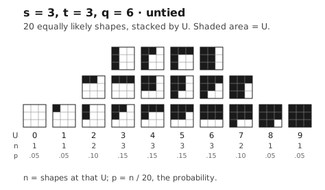
The counting can be drawn. Give each S score a column and each T score a row, and shade a cell when that S score is below that T score: the shaded area is U. Reading the scores from lowest to highest traces a path across the grid from bottom left to top right, one step right for each S score and one step up for each T score, and everything to the left of the path is shaded. Stack every possible path by its U value and the stacks are the null distribution. Here are all 20 paths for two groups of three with no tied scores. These counts are the classical Mann–Whitney distribution, and under each column are its count and its probability.

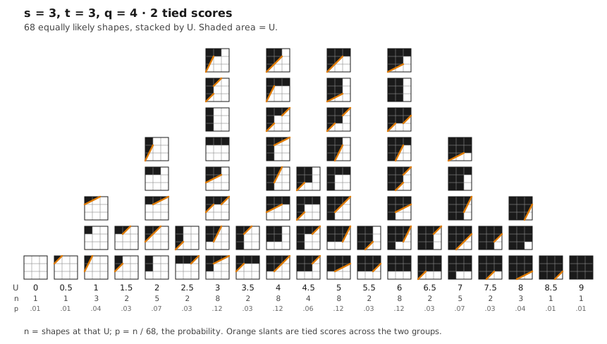
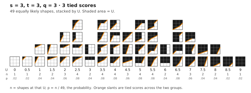
Twenty small 3 by 3 lattices stacked in columns by U from 0 to 9; column heights 1, 1, 2, 3, 3, 3, 3, 2, 1, 1. — s = 3, t = 3, q = 6: six steps for six people, so no tied scores.

Tied scores change the picture. Scores that share a value are crossed in a single step, so a path through n scores with tied scores has fewer than n steps: q counts the steps, and q = n means no tied scores at all. When S and T scores share a value, that step is a slant across their cells, shown in orange. The slant cuts the cells where scores tie in half, so the shaded area is still exactly U, and can now land on halves. Different orders that trace the same picture count once: it is the distinct shapes that are equally likely. With q = 4 (two tied scores) there are 68 shapes, and with q = 3 (three tied scores) there are 49, each with its own distribution.

Sixty-eight small 3 by 3 lattices, most with orange slants, stacked in columns by U from 0 to 9 in steps of a half. — s = 3, t = 3, q = 4: four steps for six people, so two tied scores.

Forty-nine small 3 by 3 lattices, most with orange slants, stacked in columns by U from 0 to 9 in steps of a half. — s = 3, t = 3, q = 3: three steps for six people, so three tied scores.

The site holds these counts, computed exactly in advance, for every pair of group sizes up to 20 × 20 and every possible q: about 1.3 million exact whole numbers. What it can't know is which q applies to the population you sampled from, so NXV averages over the possibilities. The number of tied scores has a floor set by the pigeonhole principle (n − r, when there are more people than scale points) and a ceiling of n − 1. Each possibility in between is weighted by a Poisson distribution with mean λ, cut to that range.

The Poisson distribution is the standard model for counts of rare, independent events: lightning strikes in a county over a summer, or the calls a nurse gets during a night on call. Using it for tied scores treats them as arising independently, by chance. If tied scores in your data are not independent, for instance because people cluster on a score for a reason, that clustering is itself part of what is being measured. The weighted average gives a single exact distribution of U, and pNXV is its total probability in the tail at or beyond the U you observed; for a two-tailed test, both tails, everything at least as far from the middle as your U. The paper gives the full construction and the proofs.